Statistical Inference: Hypothesis Testing#
This is Part 2 of statistical inference, building directly on the foundation in Chapter 9. Where Chapter 9 was about estimation — using a sample to put a sensible range on a population parameter — this chapter is about decision-making: using a sample to answer yes/no questions about a population.
For example:
Is the proportion of students who support extending library hours different from 50%?
Is the average birth weight of smokers’ babies different from non-smokers’ babies?
Did students score differently on the reading and writing exams?
Each of those is a hypothesis test. The framework is always the same — we’ll see it in detail below — and we just plug in different formulas for different kinds of data (proportions, means, paired samples).
Setting Up#
If you want to follow along in your own notebook (Jupyter, Colab, or anywhere else), import these libraries first. We’ll use them throughout the chapter — proportion tests live in statsmodels, t-tests in scipy.stats, and the CI helpers in both:
import numpy as np
import pandas as pd
from scipy import stats
from scipy.stats import ttest_ind, ttest_1samp, ttest_rel
from statsmodels.stats.proportion import proportions_ztest, proportion_confint
import matplotlib.pyplot as plt
Tip
statsmodels ships with Anaconda by default. If you’re on a fresh Python install and the from statsmodels... line errors, run !pip install statsmodels in a cell first.
Hypothesis Testing: The Framework#
Confidence intervals tell us how precise our estimates are. But what if we want to answer a yes/no question: “Is the rate of premature births really different between smokers and nonsmokers, or could the difference just be due to chance?”
That’s what hypothesis testing does — it gives us a rigorous, repeatable way to make decisions about whether an observed difference is real.
The Logic (It Feels Backwards at First)#
Hypothesis testing follows a specific logic that might seem strange the first time you see it:
Assume there’s no effect (the “null hypothesis”)
Calculate how likely we’d see our data if this assumption were true
If it’s very unlikely, reject the assumption and conclude there IS an effect
Think of it like a courtroom: we assume the defendant is innocent (null hypothesis) until the evidence is overwhelming enough to conclude guilt (reject the null). We never “prove innocence” — we either find enough evidence to convict, or we don’t.
Key Terms#
Here are the terms you need to know. Don’t worry if they feel abstract right now — we’ll work through concrete examples shortly:
Term |
Definition |
Example |
|---|---|---|
Null Hypothesis (H₀) |
The “no effect” assumption |
“There’s no difference between the two groups” |
Alternative Hypothesis (H₁) |
What we’re trying to show |
“There IS a difference between the two groups” |
p-value |
Probability of seeing our data (or more extreme) if H₀ is true |
p = 0.03 means 3% chance |
Significance Level (α) |
Our threshold for “unlikely enough” |
Typically α = 0.05 (5%) |
Test Statistic |
A number summarising how far our data is from H₀ |
t-statistic, z-score |
The Decision Rule#
The decision is straightforward — compare the p-value to your chosen significance level:
p-value |
Decision |
Interpretation |
|---|---|---|
p < α |
Reject H₀ |
Evidence of a difference (statistically significant) |
p ≥ α |
Fail to reject H₀ |
No evidence of a difference |
Visually, this is what the rejection region looks like for a two-tailed test at α = 0.05. If our test statistic lands in either red tail, we reject H₀; if it lands anywhere in the blue middle, we fail to reject:
Show code cell source
x = np.linspace(-4, 4, 400)
y = stats.norm.pdf(x)
z_critical = 1.96

fig, ax = plt.subplots(figsize=(10, 5))
ax.plot(x, y, color='steelblue', linewidth=2)

# Fail-to-reject region (middle)
ax.fill_between(x, y, where=(x >= -z_critical) & (x <= z_critical),
                alpha=0.25, color='steelblue', label='Fail to reject H₀ (95%)')

# Rejection regions (tails)
ax.fill_between(x, y, where=(x <= -z_critical),
                alpha=0.6, color='crimson', label='Reject H₀ (5% total: 2.5% + 2.5%)')
ax.fill_between(x, y, where=(x >= z_critical),
                alpha=0.6, color='crimson')

# Critical-value lines
ax.axvline(x=-z_critical, color='crimson', linestyle='--', alpha=0.7)
ax.axvline(x=z_critical, color='crimson', linestyle='--', alpha=0.7)

# Critical-value labels (with white background so they don't clash with the dashed line)
label_kwargs = dict(ha='center', color='crimson', fontsize=11,
                    bbox=dict(facecolor='white', edgecolor='none', pad=2))
ax.text(-z_critical, -0.02, "−" + str(z_critical), **label_kwargs)
ax.text(z_critical, -0.02, "+" + str(z_critical), **label_kwargs)

ax.set_xlabel('Test statistic (z)')
ax.set_ylabel('Density (under H₀)')
ax.set_title('Rejection region for a two-tailed test at α = 0.05')
ax.legend(loc='upper right')
ax.set_ylim(-0.04, 0.45)
plt.tight_layout()
plt.show()
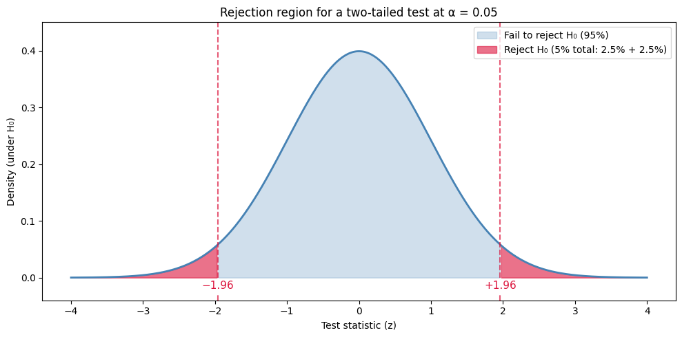
Two things to notice. First, the rejection region is just the 5% of the area split between the two tails (2.5% in each). Second, the cutoff values ±1.96 are the same z-scores we computed in Chapter 9 with stats.norm.ppf(0.975) — we’ll use them constantly.
Warning
“Fail to reject H₀” is NOT the same as “accept H₀”! This is one of the most common mistakes in statistics. We never prove the null hypothesis is true — we just don’t have enough evidence to reject it. It’s like saying “not guilty” in court — it doesn’t mean “innocent”, just that the evidence wasn’t strong enough.
Hypothesis Test for One Proportion (Z-Test)#
The simplest hypothesis test asks: is one group’s proportion different from a known baseline? For example: “Out of all students surveyed, is the percentage who support a policy different from 50%?” The baseline (here, 50%) is fixed — we’re testing whether the observed proportion strays meaningfully from it.
Note
Example: extending library hours. A university surveyed 200 students about whether they support extending library hours to 24/7 during exam period (1 = yes, 0 = no).
Research question: Is the proportion of students who support the extension different from 50%?
H₀: p = 0.50 (students are evenly split)
H₁: p ≠ 0.50 (the proportion differs from 50%)
Significance level: α = 0.05
The Formula#
For a one-proportion test, the formula is simpler than the two-proportion case — we’re just comparing one observed proportion to a hypothesised value:
The numerator is how far the sample proportion lands from the hypothesised value. The denominator is the standard error assuming H₀ is true — that’s why p_0 (not p̂) appears under the square root.
Example Walkthrough#
Step 1 — Load the data and compute the sample proportion:
df = pd.read_csv("https://raw.githubusercontent.com/sakibanwar/python-notes/main/data/library_survey.csv")

n = len(df)
x = df["support"].sum()        # number of "yes" responses
p_hat = x / n

print("Sample size n =", n)
print("Number who support x =", x)
print("Sample proportion p_hat =", round(p_hat, 4))
Sample size n = 200
Number who support x = 110
Sample proportion p_hat = 0.55
So 110 of 200 students (55%) said yes. Is that meaningfully different from 50%, or could the gap just be sampling noise?
Step 2 — Check the conditions. The z-test relies on the sampling distribution of p̂ being approximately normal. The standard rule of thumb is the success–failure condition: under H₀ we need at least 10 expected “yes” responses and at least 10 expected “no” responses:
p_0 = 0.50

print("n * p_0       =", int(n * p_0),       "(need >= 10)")
print("n * (1 - p_0) =", int(n * (1 - p_0)), "(need >= 10)")
print("Both conditions satisfied?", n * p_0 >= 10 and n * (1 - p_0) >= 10)
n * p_0       = 100 (need >= 10)
n * (1 - p_0) = 100 (need >= 10)
Both conditions satisfied? True
Both checks pass comfortably (100 expected yes, 100 expected no), so the normal approximation is fine here.
Step 3 — Run the z-test. Rather than calculating z and p by hand, we use proportions_ztest from statsmodels. The function takes four arguments:
count— the number of successes in the sample (herex, the count of “yes” responses).nobs— the total number of observations (heren).value— the hypothesised proportion under H₀ (here0.50).alternative—"two-sided","larger", or"smaller"— must match your H₁.
It returns the test statistic and the p-value as a tuple:
z_stat, p_value = proportions_ztest(count=x, nobs=n, value=p_0, alternative="two-sided")

print("z-statistic =", round(z_stat, 4))
print("p-value     =", round(p_value, 4))
z-statistic = 1.4213
p-value     = 0.1552
A z-statistic of about 1.42 is well inside the ±1.96 fail-to-reject region we plotted earlier — that already tells us the data isn’t compelling enough to reject H₀.
Step 4 — Confidence interval. The companion function proportion_confint gives the 95% CI in one line. Its arguments:
count,nobs— same as before.alpha—1 − confidence level, so0.05for a 95% CI,0.01for a 99% CI.method— how to compute the interval."normal"is the standard Wald formulap̂ ± z* × SEwe used in Chapter 9.
It returns a (lower, upper) tuple:
ci_lower, ci_upper = proportion_confint(count=x, nobs=n, alpha=0.05, method="normal")

print("95% CI for p: (", round(ci_lower, 4), ",", round(ci_upper, 4), ")")
print("Does the CI contain 0.50?", ci_lower <= p_0 <= ci_upper)
95% CI for p: ( 0.4811 , 0.6189 )
Does the CI contain 0.50? True
The CI (0.481, 0.619) contains 0.50, which agrees with the test: 50% is a plausible value for the true population proportion.
Step 5 — Decision and conclusion.
alpha = 0.05

if p_value < alpha:
    print("p-value", round(p_value, 4), "< α", alpha, ": REJECT H₀")
else:
    print("p-value", round(p_value, 4), ">= α", alpha, ": FAIL TO REJECT H₀")
p-value 0.1552 >= α 0.05 : FAIL TO REJECT H₀
So we fail to reject H₀. Putting it into the kind of sentence you’d use in a write-up:
There is not sufficient evidence at the 5% significance level to conclude that the proportion of students who support extended library hours differs from 50% (z = 1.42, p = 0.155, 95% CI [0.481, 0.619]).
Notice three things:
The test and the CI agree. They have to: a 95% CI containing the null value is mathematically equivalent to a two-tailed test failing to reject at α = 0.05.
A “fail to reject” verdict is not the same as “we proved students are evenly split”. 55% really might be the true rate; we just don’t have enough evidence to claim it differs from 50%.
A larger sample would shrink the standard error and could turn this borderline result either way — so reporting the CI alongside the p-value is more honest than the p-value alone.
Hypothesis Test for Two Proportions (Z-Test)#
The next case up: instead of comparing one proportion to a fixed baseline, we compare two proportions to each other. Both groups give us their own observed rate (p̂₁ and p̂₂), and we ask whether the gap between them is real or just sampling noise.
Note
Example: premature births and smoking. The births_smoking.csv dataset has 1,000 births with a habit column (nonsmoker or smoker) and a premature flag (1 = premature, 0 = full term).
Research question: Does the premature birth rate differ between smokers and nonsmokers?
H₀: p₁ = p₂ (the rates are equal)
H₁: p₁ ≠ p₂ (the rates differ)
Significance level: α = 0.05
The Formula#
The z-statistic measures how many standard errors the observed difference is from zero:
The standard error uses the pooled proportion — the overall proportion assuming H₀ is true (i.e., treating both groups as one big group):
Why pool? Because under H₀ there’s no real difference between the groups — so our best estimate of the common rate combines all the data. (For confidence intervals we’ll unpool the SE; we’ll see why in Step 4.)
Example Walkthrough#
Step 1 — Load the data and compute the per-group proportions. A single groupby gives us the counts and totals we need:
births = pd.read_csv("https://raw.githubusercontent.com/sakibanwar/python-notes/main/data/births_smoking.csv")

# Get total births and number premature in each group
counts = births.groupby("habit")["premature"].agg(["sum", "count"])
print(counts)
print()

# Pull out the numbers we need
n1 = counts.loc["nonsmoker", "count"]
x1 = counts.loc["nonsmoker", "sum"]
n2 = counts.loc["smoker", "count"]
x2 = counts.loc["smoker", "sum"]

# Per-group premature rates
p1 = x1 / n1
p2 = x2 / n2

print("Nonsmoker premature rate:", round(p1, 4), "= about", round(p1 * 100, 1), "%")
print("Smoker premature rate:   ", round(p2, 4), "= about", round(p2 * 100, 1), "%")
print("Observed difference (p1 - p2):", round(p1 - p2, 4))
           sum  count
habit
nonsmoker  110    800
smoker      42    200

Nonsmoker premature rate: 0.1375 = about 13.8 %
Smoker premature rate:    0.21 = about 21.0 %
Observed difference (p1 - p2): -0.0725
So smokers have a 21.0% premature rate compared to 13.75% for nonsmokers — a 7.25 percentage-point gap. Is this difference statistically significant, or could it be sampling noise?
Step 2 — Check the conditions. Same success–failure rule as before, but now applied to each group. Under H₀ both groups share the pooled proportion p̂_pool, so we need at least 10 expected successes and 10 expected failures in each group:
p_pool = (x1 + x2) / (n1 + n2)

print("Pooled proportion p̂_pool =", round(p_pool, 4))
print()
print("Group 1 (nonsmokers): n1 * p_pool =", round(n1 * p_pool, 1), ", n1 * (1 - p_pool) =", round(n1 * (1 - p_pool), 1))
print("Group 2 (smokers):    n2 * p_pool =", round(n2 * p_pool, 1), ", n2 * (1 - p_pool) =", round(n2 * (1 - p_pool), 1))
Pooled proportion p̂_pool = 0.152

Group 1 (nonsmokers): n1 * p_pool = 121.6 , n1 * (1 - p_pool) = 678.4
Group 2 (smokers):    n2 * p_pool = 30.4 , n2 * (1 - p_pool) = 169.6
All four expected counts comfortably exceed 10, so the normal approximation is fine.
Step 3 — Run the z-test. The same proportions_ztest function we used before handles two-proportion comparisons too — we just hand it a list of two counts and a list of two sample sizes (no value= needed; the null is automatically “p₁ = p₂”):
z_stat, p_value = proportions_ztest(count=[x1, x2], nobs=[n1, n2], alternative="two-sided")

print("z-statistic =", round(z_stat, 4))
print("p-value     =", round(p_value, 4))
z-statistic = -2.5543
p-value     = 0.0106
A z-statistic of about −2.55 sits well outside the ±1.96 fail-to-reject region we plotted earlier — already a strong hint we’ll reject H₀.
Step 4 — Confidence interval for the difference. The CI uses the unpooled SE (because we no longer assume the rates are equal — we want the most honest estimate of the gap):
diff = p1 - p2
se_unpooled = np.sqrt(p1*(1 - p1)/n1 + p2*(1 - p2)/n2)
z_critical = stats.norm.ppf(0.975)   # 1.96 for a 95% CI

ci_lower = diff - z_critical * se_unpooled
ci_upper = diff + z_critical * se_unpooled

print("95% CI for (p1 - p2): (", round(ci_lower, 4), ",", round(ci_upper, 4), ")")
print("Does the CI contain 0?", ci_lower <= 0 <= ci_upper)
95% CI for (p1 - p2): ( -0.1338 , -0.0112 )
Does the CI contain 0? False
The CI is roughly (−0.134, −0.011) and does not contain 0 — that agrees with the test rejecting H₀.
Step 5 — Decision and conclusion.
alpha = 0.05

if p_value < alpha:
    print("p-value", round(p_value, 4), "< α", alpha, ": REJECT H₀")
else:
    print("p-value", round(p_value, 4), ">= α", alpha, ": FAIL TO REJECT H₀")
p-value 0.0106 < α 0.05 : REJECT H₀
So we reject H₀. Writing it up properly:
There is sufficient evidence at the 5% significance level to conclude that the premature birth rate differs between smokers and nonsmokers (z = −2.55, p = 0.011, 95% CI for the difference [−0.134, −0.011]). Smokers in this sample had a higher premature rate (21.0% vs 13.75% for nonsmokers).
Notice three things:
The test and the CI agree — the CI excludes 0 if and only if the two-tailed test rejects at α = 0.05.
We pool for the test (because under H₀ the rates are assumed equal) but unpool for the CI (because we want an honest estimate of the gap, not assuming H₀).
“Significant” means real, not necessarily important. A 7.25 percentage-point difference in premature birth rates is also clinically meaningful — but always check that yourself; the test alone won’t tell you.
Tip
Same function, different argument shape. proportions_ztest recognises a one-proportion test when you pass scalar count and nobs plus a value=p_0, and a two-proportion test when you pass a list of two counts and a list of two sample sizes (no value needed — the null is “p₁ = p₂”). The interface is intentionally consistent so you don’t need to remember a separate function for each case.
Hypothesis Test for One Mean (t-Test)#
We’ve been testing proportions (yes/no outcomes). What if our outcome is a measurement — a birth weight, an exam score, the number of cars on a road? Then we need a t-test instead of a z-test.
The simplest case: we have one group’s measurements, and we want to test whether the population mean equals some hypothesised value μ₀.
Note
Example: Friday the 13th. A folk superstition says Friday the 13th is “unlucky” — quieter roads, fewer shoppers, more accidents. The dataset friday.csv records pairs of activity (traffic, shopping, hospital accidents) on Friday the 6th and Friday the 13th of the same month, across multiple months. The column diff is defined as:
diff= (activity on the 6th) − (activity on the 13th)
A positive diff means more activity on the 6th (people stayed home on the 13th). A negative diff means the opposite.
Research question: Is there a systematic difference in activity between the 6th and the 13th?
H₀: μ_diff = 0 (no average difference)
H₁: μ_diff ≠ 0 (there is a difference)
Significance level: α = 0.05
The Formula#
For a one-sample t-test, the test statistic is:
Reading top to bottom:
the numerator is how far the sample mean lies from the hypothesised value
μ₀,the denominator is the standard error — the SE of the sample mean we built up in Chapter 9.
We use the t-distribution (not the normal) because we’re estimating σ from the sample. Degrees of freedom are n − 1. As n grows, t* converges toward z* (recall the z-vs-t note from Chapter 9).
Example Walkthrough#
Step 1 — Load the data and inspect the differences.
df = pd.read_csv("https://raw.githubusercontent.com/sakibanwar/python-notes/main/data/friday.csv")
df.head()
| type | date | sixth | thirteenth | diff | location | |
|---|---|---|---|---|---|---|
| 0 | traffic | 1990, July | 139246 | 138548 | 698 | 7 to 8 |
| 1 | traffic | 1990, July | 134012 | 132908 | 1104 | 9 to 10 |
| 2 | traffic | 1991, September | 137055 | 136018 | 1037 | 7 to 8 |
| 3 | traffic | 1991, September | 133732 | 131843 | 1889 | 9 to 10 |
| 4 | traffic | 1991, December | 123552 | 121641 | 1911 | 7 to 8 |
Each row is one paired measurement: a type of activity (traffic, shopping, accident), a date, the values on the 6th and the 13th, and the diff. We’ll work directly with the diff column:
diff = df["diff"]

print("n =", len(diff))
print("mean of diff:", round(diff.mean(), 2))
print("std of diff (ddof=1):", round(diff.std(ddof=1), 2))
n = 61
mean of diff: 266.33
std of diff (ddof=1): 849.18
The sample mean is positive (about +266), suggesting more activity on the 6th on average. But the standard deviation is enormous (≈849) — could that mean just be noise?
Step 2 — Check the conditions. A one-sample t-test is robust when the sample is either roughly normal or large enough (n ≥ 30) for the CLT to kick in:
print("n =", len(diff), "(need >= 30 or roughly normal)")
n = 61 (need >= 30 or roughly normal)
n = 61 is comfortably above 30 — the test will be fine.
Step 3 — Run the t-test. scipy.stats.ttest_1samp does the whole calculation in one line. Its arguments:
first argument — the sample data (any 1-D array-like; here our
diffSeries).popmean— the hypothesised population mean μ₀ (here0).alternative(optional) —"two-sided","less", or"greater". Defaults to"two-sided".
It returns the t-statistic and a p-value:
t_stat, p_value = stats.ttest_1samp(diff, popmean=0)

print("t-statistic =", round(t_stat, 4))
print("p-value     =", round(p_value, 4))
print("df          =", len(diff) - 1)
t-statistic = 2.4495
p-value     = 0.0172
df          = 60
A t-statistic of about 2.45 says the sample mean is roughly 2.5 standard errors above zero. The p-value of 0.017 says: if there really were no average difference, we’d see a sample mean this far from zero (in either direction) only about 1.7% of the time.
Step 4 — Confidence interval. The companion function stats.t.interval gives us the 95% CI for the mean directly. Its arguments:
first argument — the confidence level (
0.95for a 95% CI).df— degrees of freedom (n − 1).loc— the centre of the interval (the sample mean).scale— the standard error (s / √n).
It returns the (lower, upper) bounds:
n = len(diff)
se = diff.std(ddof=1) / np.sqrt(n)
ci = stats.t.interval(0.95, df=n-1, loc=diff.mean(), scale=se)

print("95% CI for mean diff: (", round(ci[0], 2), ",", round(ci[1], 2), ")")
print("Does the CI contain 0?", ci[0] <= 0 <= ci[1])
95% CI for mean diff: ( 48.84 , 483.81 )
Does the CI contain 0? False
The 95% CI is roughly (48.8, 483.8), which does not contain 0 — that agrees with the test rejecting H₀.
Step 5 — Decision and conclusion.
alpha = 0.05

if p_value < alpha:
    print("p-value", round(p_value, 4), "< α", alpha, ": REJECT H₀")
else:
    print("p-value", round(p_value, 4), ">= α", alpha, ": FAIL TO REJECT H₀")
p-value 0.0172 < α 0.05 : REJECT H₀
So we reject H₀. Writing it up properly:
There is sufficient evidence at the 5% significance level to conclude that activity levels differ between Friday the 6th and Friday the 13th (t(60) = 2.45, p = 0.017, 95% CI for the mean difference [48.8, 483.8]). On average, activity was higher on the 6th than on the 13th.
Notice the parallels with everything we’ve done so far:
The test and the CI agree — the CI excludes 0 if and only if the two-tailed test rejects at α = 0.05.
The conclusion isn’t “Friday the 13th is unlucky”. It’s just that, in this sample, average activity was lower on the 13th. Whether that’s meaningful is a separate question.
The same
Estimate ± Critical × SEtemplate from Chapter 9 sits underneath everything.
Hypothesis Test for Two Means (t-Test)#
The one-sample t-test asked whether one group’s mean differed from a hypothesised value. The natural next step is to compare the means of two independent groups — for example, the average birth weight of smokers’ babies vs nonsmokers’ babies. That’s the two-sample t-test.
Note
Example: birth weight and smoking. Back to births_smoking.csv, but this time we use the weight_lbs column instead of the premature flag. We have 800 nonsmoker babies and 200 smoker babies.
Research question: Does mean birth weight differ between nonsmokers’ and smokers’ babies?
H₀: μ₁ = μ₂ (the population mean weights are equal)
H₁: μ₁ ≠ μ₂ (the population mean weights differ)
Significance level: α = 0.05
The Formula#
For a two-sample t-test the test statistic is:
The numerator is the observed gap between the two sample means. The denominator is the standard error of that gap — each group contributes its own variance divided by its sample size. We use Welch’s version, which doesn’t assume the two groups have equal variances (the recommended default — see the note below).
Example Walkthrough#
Step 1 — Load the data and split into the two groups. The dataset is in tidy format (one row per baby, with a habit column), so splitting is just the boolean-filter pattern from Chapter 6:
births = pd.read_csv("https://raw.githubusercontent.com/sakibanwar/python-notes/main/data/births_smoking.csv")

nonsmoker_weights = births[births['habit'] == 'nonsmoker']['weight_lbs'].values
smoker_weights    = births[births['habit'] == 'smoker']['weight_lbs'].values

print("Nonsmokers: n =", len(nonsmoker_weights), ", mean =", round(nonsmoker_weights.mean(), 3), "lbs")
print("Smokers:    n =", len(smoker_weights),    ", mean =", round(smoker_weights.mean(), 3),    "lbs")
print("Observed difference:", round(nonsmoker_weights.mean() - smoker_weights.mean(), 3), "lbs")
Nonsmokers: n = 800 , mean = 7.19 lbs
Smokers:    n = 200 , mean = 6.892 lbs
Observed difference: 0.297 lbs
There’s about a 0.3 lb difference — but is that gap real or just sampling noise?
Step 2 — Check the conditions. A two-sample t-test is robust when each sample is either roughly normal or large enough (n ≥ 30) for the CLT to kick in:
print("Nonsmokers n =", len(nonsmoker_weights), "(need >= 30 or roughly normal)")
print("Smokers    n =", len(smoker_weights),    "(need >= 30 or roughly normal)")
Nonsmokers n = 800 (need >= 30 or roughly normal)
Smokers    n = 200 (need >= 30 or roughly normal)
Both samples are well above 30 — the test will be fine.
Step 3 — Run the t-test. scipy.stats.ttest_ind (the “ind” stands for independent samples) does the whole calculation in one line. Its arguments:
two array arguments — the two samples to compare (order doesn’t change the conclusion, only the sign of
t).equal_var(optional) — whether to assume equal variances. Defaults toFalse, giving Welch’s t-test (the recommended default — see the note below).alternative(optional) —"two-sided","less", or"greater". Defaults to"two-sided".
It returns the t-statistic and a p-value:
t_stat, p_value = ttest_ind(nonsmoker_weights, smoker_weights)

print("t-statistic =", round(t_stat, 4))
print("p-value     =", round(p_value, 6))
t-statistic = 2.8687
p-value     = 0.004209
A t-statistic of about 2.87 sits well outside the ±1.96 cutoff. The p-value of about 0.004 says: if there really were no average difference, we’d see a sample gap this large only about 0.4% of the time — well under our α = 0.05 threshold.
Note
By default, ttest_ind() performs Welch’s t-test, which does NOT assume the two groups have equal variances. This is the recommended default — it’s more robust. If you specifically need the pooled (Student’s) t-test, use ttest_ind(a, b, equal_var=True), but Welch’s is almost always the better choice.
Step 4 — Confidence interval. Same stats.t.interval we used for the one-sample case, with two changes: the centre is the difference in means, and the scale is the combined SE. Welch’s degrees of freedom has a messy formula, but Python computes it for us in one line:
n1, n2 = len(nonsmoker_weights), len(smoker_weights)
s1 = nonsmoker_weights.std(ddof=1)
s2 = smoker_weights.std(ddof=1)

diff = nonsmoker_weights.mean() - smoker_weights.mean()
se = np.sqrt(s1**2/n1 + s2**2/n2)

# Welch–Satterthwaite degrees of freedom
df_welch = (s1**2/n1 + s2**2/n2)**2 / ((s1**2/n1)**2/(n1-1) + (s2**2/n2)**2/(n2-1))

ci_lower, ci_upper = stats.t.interval(0.95, df=df_welch, loc=diff, scale=se)

print("Welch's df:", round(df_welch, 1))
print("95% CI for (μ_nonsmoker - μ_smoker): (", round(ci_lower, 4), ",", round(ci_upper, 4), ") lbs")
print("Does the CI contain 0?", ci_lower <= 0 <= ci_upper)
Welch's df: 283.2
95% CI for (μ_nonsmoker - μ_smoker): ( 0.0788 , 0.5159 ) lbs
Does the CI contain 0? False
The CI is comfortably above zero — the gap between the two group means is positive and well-estimated, which agrees with the test rejecting H₀.
Step 5 — Decision and conclusion.
alpha = 0.05

if p_value < alpha:
    print("p-value", round(p_value, 6), "< α", alpha, ": REJECT H₀")
else:
    print("p-value", round(p_value, 6), ">= α", alpha, ": FAIL TO REJECT H₀")
p-value 0.004209 < α 0.05 : REJECT H₀
So we reject H₀. The write-up:
There is sufficient evidence at the 5% significance level to conclude that mean birth weight differs between nonsmokers’ and smokers’ babies (t ≈ 2.87, p ≈ 0.004, 95% CI for the mean difference [0.08, 0.52] lbs). Nonsmokers’ babies were on average about 0.3 lbs heavier.
Notice three things:
The test and the CI agree — the CI excludes 0 if and only if the two-tailed test rejects at α = 0.05.
The boolean-filter pattern we used to split
birthsinto two groups —births[births['habit'] == 'nonsmoker']— is exactly the same filtering you learned in Chapter 6. There’s no special “split into groups” function; the t-test just consumes two arrays.A 0.3 lb mean difference isn’t just statistically significant — it’s also clinically meaningful for neonatal health (roughly 135 grams, enough to matter). That’s the kind of side check we’ll discuss in the next section.
Hypothesis Test for Paired Means (Paired t-Test)#
So far our t-tests have used independent samples — different people in each group. But sometimes the two measurements come from the same subject: a before/after measurement, two test scores per student, the same patient on two drugs. These observations are paired, and treating them as independent throws away useful information.
The fix is the paired t-test. And it has a beautiful property: it’s actually just a one-sample t-test on the differences — the same thing we did with the Friday-the-13th data, but now applied to within-subject differences.
Note
Example: reading vs writing exams. 200 students each sat a reading test and a writing test. We want to know whether students score systematically differently on the two exams.
Research question: Do students’ mean reading and writing scores differ?
H₀: μ_diff = 0 (no average difference between reading and writing)
H₁: μ_diff ≠ 0 (there is a difference)
where diff = reading − writing for each student. Significance level: α = 0.05.
Why “Paired” Matters#
Each student’s reading and writing scores aren’t independent — students who score high on one test tend to score high on the other (overall ability, effort, fatigue, exam-taking skill). If we treated reading and writing as two independent samples and ran a two-sample t-test, that within-student correlation would inflate the standard error and make us less likely to detect a real difference.
The paired test fixes this by subtracting within each student first, then testing whether the average difference is zero. The within-student variability cancels out, giving us a more powerful test.
The Formula#
For each student, compute the difference dᵢ = readingᵢ − writingᵢ. Then test whether μ_d = 0:
This is identical to the one-sample t-test formula from the previous section, just applied to the column of differences.
Example Walkthrough#
Step 1 — Load the data and compute the differences.
df = pd.read_csv("https://raw.githubusercontent.com/sakibanwar/python-notes/main/data/reading_writing.csv")
df.head()
| student_id | reading | writing | |
|---|---|---|---|
| 0 | 1 | 61 | 56 |
| 1 | 2 | 52 | 61 |
| 2 | 3 | 70 | 65 |
| 3 | 4 | 45 | 46 |
| 4 | 5 | 69 | 71 |
Each row is one student with their two scores. The pairing is implicit: row 1 is the same student’s reading and writing scores. Take the within-student difference and inspect it:
diff = df["reading"] - df["writing"]

print("n =", len(diff))
print("mean of diff:", round(diff.mean(), 2))
print("std of diff (ddof=1):", round(diff.std(ddof=1), 2))
n = 200
mean of diff: 2.62
std of diff (ddof=1): 8.08
The mean difference is about +2.6, suggesting students score slightly higher on reading on average. With 200 students and a standard deviation of about 8, is this noise or signal?
Step 2 — Check the conditions. Once we collapse to the column of differences, the paired t-test is just a one-sample t-test, so the same condition applies: the differences should be roughly normal or the sample should be large enough (n ≥ 30):
print("n =", len(diff), "(need >= 30 or roughly normal)")
n = 200 (need >= 30 or roughly normal)
n = 200 is well above 30 — the test will be fine.
Step 3 — Run the paired t-test. scipy.stats.ttest_rel (“rel” for “related” / paired) takes:
two paired array arguments — same length, same order. Element
iof the second array is the partner of elementiof the first (here, the same student’s writing score paired with their reading score).
It computes the differences a − b internally and runs a one-sample t-test against zero:
t_stat, p_value = stats.ttest_rel(df["reading"], df["writing"])

print("t-statistic =", round(t_stat, 4))
print("p-value     =", round(p_value, 6))
print("df          =", len(df) - 1)
t-statistic = 4.5957
p-value     = 8e-06
df          = 199
A t-statistic of about 4.6 sits far outside the ±1.96 cutoff. The p-value is essentially 0 — if there really were no average difference, we’d be vanishingly unlikely to see this much.
Step 4 — The key insight. A paired t-test is literally a one-sample t-test on the differences. Watch:
# Same calculation, two different ways of expressing it
t_paired,    p_paired     = stats.ttest_rel(df["reading"], df["writing"])
t_onesample, p_onesample  = stats.ttest_1samp(diff, popmean=0)

print("ttest_rel:    t =", round(t_paired, 4),    " p =", round(p_paired, 6))
print("ttest_1samp:  t =", round(t_onesample, 4), " p =", round(p_onesample, 6))
ttest_rel:    t = 4.5957  p = 8e-06
ttest_1samp:  t = 4.5957  p = 8e-06
Identical numbers. They’re the same test. ttest_rel is just a convenience that subtracts the columns for you and saves a line of code.
Step 5 — Confidence interval. Same stats.t.interval we used for the one-sample case, applied to the differences:
n = len(diff)
se = diff.std(ddof=1) / np.sqrt(n)
ci = stats.t.interval(0.95, df=n-1, loc=diff.mean(), scale=se)

print("95% CI for mean diff: (", round(ci[0], 2), ",", round(ci[1], 2), ")")
print("Does the CI contain 0?", ci[0] <= 0 <= ci[1])
95% CI for mean diff: ( 1.5 , 3.75 )
Does the CI contain 0? False
The CI is roughly (1.5, 3.75) — clearly above zero — which agrees with the test rejecting H₀.
Step 6 — Decision and conclusion.
alpha = 0.05

if p_value < alpha:
    print("p-value", round(p_value, 6), "< α", alpha, ": REJECT H₀")
else:
    print("p-value", round(p_value, 6), ">= α", alpha, ": FAIL TO REJECT H₀")
p-value 8e-06 < α 0.05 : REJECT H₀
So we reject H₀. The write-up:
There is sufficient evidence at the 5% significance level to conclude that students score differently on reading and writing exams (paired t(199) = 4.60, p < 0.001, 95% CI for the mean difference [1.5, 3.75]). On average, reading scores are about 2.6 points higher than writing scores.
Tip
When should I use paired vs two-sample? If each observation in group 1 has a natural partner in group 2 — same student, same patient, before/after — use paired (ttest_rel). If the two groups are independent people/units, use two-sample (ttest_ind). Mixing them up is one of the most common mistakes in applied statistics: treating paired data as independent inflates the standard error and reduces your power to detect real effects.
Statistical Significance vs Practical Significance#
We’ve been focused on p-values and statistical significance. But here’s something crucial that many people miss: a result can be statistically significant without being practically important.
The Problem with Large Samples#
Why? Because with a very large sample, even tiny differences become statistically significant. Watch what happens:
# Large sample with tiny difference — 10,000 observations per group
stat_practical = pd.read_csv("https://raw.githubusercontent.com/sakibanwar/python-notes/main/data/stat_vs_practical.csv")
group_1 = stat_practical[stat_practical['group'] == 'Group A']['score'].values
group_2 = stat_practical[stat_practical['group'] == 'Group B']['score'].values

t_stat, p_value = ttest_ind(group_1, group_2)
print("Difference in means:", round(group_2.mean() - group_1.mean(), 2))
print("p-value:", round(p_value, 6))
Difference in means: 0.51
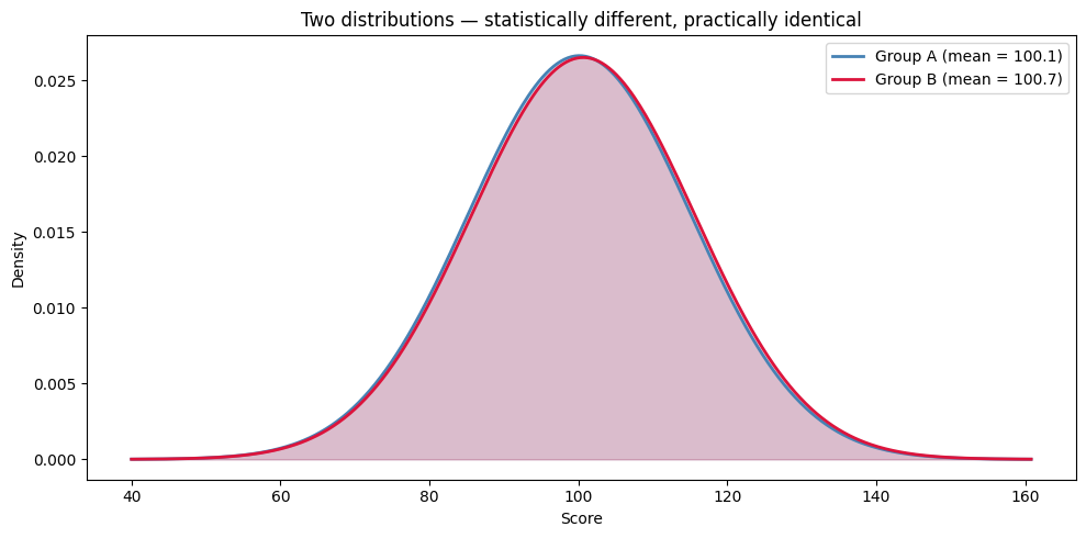
p-value: 0.016266
The result is “significant” (p < 0.05), but the actual difference is only about half a point on a scale where the standard deviation is 15. The picture makes that distinction stark — the two distributions are almost completely on top of each other, even though the test confidently rejects H₀:
Show code cell source
mean1, std1 = group_1.mean(), group_1.std(ddof=1)
mean2, std2 = group_2.mean(), group_2.std(ddof=1)

x = np.linspace(min(mean1, mean2) - 4*max(std1, std2),
                max(mean1, mean2) + 4*max(std1, std2), 500)

fig, ax = plt.subplots(figsize=(10, 5))
ax.plot(x, stats.norm.pdf(x, mean1, std1), color='steelblue', linewidth=2,
        label='Group A (mean = ' + str(round(mean1, 1)) + ')')
ax.plot(x, stats.norm.pdf(x, mean2, std2), color='crimson', linewidth=2,
        label='Group B (mean = ' + str(round(mean2, 1)) + ')')
ax.fill_between(x, stats.norm.pdf(x, mean1, std1), alpha=0.2, color='steelblue')
ax.fill_between(x, stats.norm.pdf(x, mean2, std2), alpha=0.2, color='crimson')
ax.set_xlabel('Score')
ax.set_ylabel('Density')
ax.set_title('Two distributions — statistically different, practically identical')
ax.legend()
plt.tight_layout()
plt.show()
Would you change a business decision based on a difference this tiny? Probably not.
This is why you should always ask two questions, not just one:
Is the difference statistically significant? (What the p-value tells you)
Is the difference big enough to matter? (What the p-value does NOT tell you)
Always Report Both#
When reporting results, good practice is to state three things:
Whether the result is statistically significant (the p-value)
The size of the effect (the actual difference in means or proportions)
Whether the effect matters practically (your judgement, based on context)
For example, here’s how you might write up our birth weight findings:
“Nonsmoking mothers had babies weighing on average about 0.3 lbs more than smoking mothers (7.19 vs 6.89 lbs). This difference was statistically significant (t = 2.87, p = 0.004). A roughly 135-gram gap in birth weight is also clinically meaningful, as it can affect neonatal health outcomes.”
Notice how this reports the actual numbers, the statistical test, AND the practical interpretation.
Tip
Always interpret your results in context. Ask yourself: “Even though this is statistically significant, does the difference actually matter in the real world?” A p-value tells you whether the difference is real, not whether it’s important.
One-Tailed vs Two-Tailed Tests#
By default, all the tests we’ve been running are two-tailed — they check for a difference in either direction. But sometimes you have a specific directional hypothesis. For example, you don’t just think smokers are different — you specifically think smokers have lower birth weights.
Two-Tailed Test (Default)#
H₀: μ₁ = μ₂
H₁: μ₁ ≠ μ₂ (could be higher OR lower)
One-Tailed Test#
H₀: μ₁ ≥ μ₂
H₁: μ₁ < μ₂ (specifically testing if one group is lower)
The two cases differ in where the rejection region sits. Side by side:
Show code cell source
x = np.linspace(-4, 4, 400)
y = stats.norm.pdf(x)

fig, axes = plt.subplots(1, 2, figsize=(14, 4.5), sharey=True)

# Two-tailed
ax = axes[0]
ax.plot(x, y, color='steelblue', linewidth=2)
ax.fill_between(x, y, where=(x <= -1.96), alpha=0.6, color='crimson', label='Reject (2.5%)')
ax.fill_between(x, y, where=(x >=  1.96), alpha=0.6, color='crimson')
ax.fill_between(x, y, where=(x >= -1.96) & (x <= 1.96), alpha=0.2, color='steelblue', label='Fail to reject (95%)')
ax.axvline(-1.96, color='crimson', linestyle='--', alpha=0.7)
ax.axvline( 1.96, color='crimson', linestyle='--', alpha=0.7)
ax.set_title('Two-tailed: 5% split between two tails\nCutoffs at ±1.96')
ax.set_xlabel('Test statistic')
ax.set_ylabel('Density')
ax.legend(loc='upper right', fontsize=9)

# One-tailed (upper)
ax = axes[1]
ax.plot(x, y, color='steelblue', linewidth=2)
ax.fill_between(x, y, where=(x >= 1.645), alpha=0.6, color='crimson', label='Reject (5%)')
ax.fill_between(x, y, where=(x <  1.645), alpha=0.2, color='steelblue', label='Fail to reject (95%)')
ax.axvline(1.645, color='crimson', linestyle='--', alpha=0.7)
ax.set_title('One-tailed (upper): 5% all in one tail\nCutoff at +1.645')
ax.set_xlabel('Test statistic')
ax.legend(loc='upper right', fontsize=9)

plt.tight_layout()
plt.show()
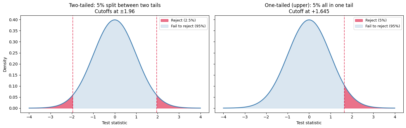
Notice the lower cutoff for the one-tailed case: 1.645 vs 1.96. That’s why one-tailed tests are more “powerful” — a smaller test statistic suffices to reject. But the cost is that you can’t reject in the other direction at all. The test is blind to evidence pointing the wrong way.
How do you convert? Since ttest_ind always returns a two-tailed p-value, you simply divide by 2:
# For a one-tailed test, divide the two-tailed p-value by 2
# (only valid if the observed difference is in the expected direction)

t_stat, p_value_two_tailed = ttest_ind(smoker_weights, nonsmoker_weights)
p_value_one_tailed = p_value_two_tailed / 2

print("Two-tailed p-value:", round(p_value_two_tailed, 4))
print("One-tailed p-value:", round(p_value_one_tailed, 4))
Two-tailed p-value: 0.0042
One-tailed p-value: 0.0021
Warning
One-tailed tests are more powerful (more likely to detect an effect), which makes them tempting. But they should only be used when you had a clear directional hypothesis before looking at the data. If you choose the direction after seeing the results, you’re cheating — and your p-value is no longer valid. When in doubt, use the two-tailed test.
Understanding p-Values More Deeply#
The p-value is one of the most commonly used — and most commonly misunderstood — concepts in statistics. Let’s be really clear about what it does and doesn’t tell you.
What the p-Value IS#
The p-value is the probability of observing data as extreme as (or more extreme than) what we got, assuming the null hypothesis is true.
A p-value of 0.03 means: “If there really were no effect, we’d see results this extreme only 3% of the time.” That’s pretty unlikely — so we take it as evidence against the null.
Geometrically, the p-value is literally the area under the curve beyond the observed test statistic. For a two-sided test, it’s the area in both tails:
Show code cell source
x = np.linspace(-4, 4, 400)
y = stats.norm.pdf(x)
t_obs = 2.0   # an example observed test statistic

fig, ax = plt.subplots(figsize=(10, 5))
ax.plot(x, y, color='steelblue', linewidth=2)
ax.fill_between(x, y, where=(x >=  t_obs), alpha=0.6, color='crimson',
                label='p-value = total shaded area\n(both tails for a two-sided test)')
ax.fill_between(x, y, where=(x <= -t_obs), alpha=0.6, color='crimson')
ax.axvline( t_obs, color='crimson', linestyle='--', alpha=0.7)
ax.axvline(-t_obs, color='crimson', linestyle='--', alpha=0.7)
ax.text( t_obs, -0.025, "+t_obs", ha='center', color='crimson', fontsize=11,
        bbox=dict(facecolor='white', edgecolor='none', pad=2))
ax.text(-t_obs, -0.025, "−t_obs", ha='center', color='crimson', fontsize=11,
        bbox=dict(facecolor='white', edgecolor='none', pad=2))
ax.set_xlabel('Test statistic (under H₀)')
ax.set_ylabel('Density')
ax.set_title('What the p-value IS: the tail area beyond the observed test statistic')
ax.legend(loc='upper right')
ax.set_ylim(-0.04, 0.45)
plt.tight_layout()
plt.show()
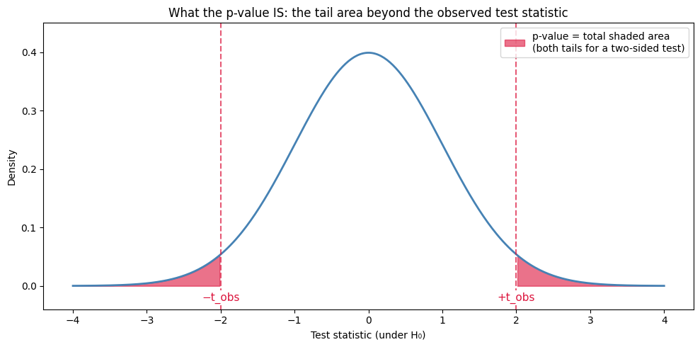
So when proportions_ztest or ttest_ind returns p_value = 0.03, it’s saying “the red shaded area sums to 0.03”. The smaller that area, the further t_obs is out into the tail, and the more incompatible our data is with H₀.
What the p-Value is NOT#
This table is worth memorising — these mistakes appear in published research papers, news articles, and even some textbooks:
Wrong Interpretation |
Why It’s Wrong |
|---|---|
“There’s a 3% chance the null is true” |
The p-value says nothing about the probability that H₀ is true |
“There’s a 97% chance the alternative is true” |
The p-value doesn’t give probabilities of hypotheses being true or false |
“The effect is important/large” |
The p-value measures evidence, not effect size (remember our large-sample example!) |
“The results are definitely real” |
Low p-values can still be false positives — a 5% significance level means you’ll be wrong about 1 in 20 times |
The Universal Workflow#
Look back at the five tests in this chapter — one-proportion, two-proportion, one-sample t, two-sample t, paired t. Different formulas, different functions, different scenarios. But the shape of every example was the same:
Step |
What you do |
Where it shows up |
|---|---|---|
1. State the question |
Identify what you’re comparing and write H₀ and H₁. Pick α. |
The |
2. Load and explore |
Read the CSV, look at |
First couple of code cells |
3. Check conditions |
For proportion tests, the success–failure rule. For t-tests, n ≥ 30 or roughly normal data. |
A small |
4. Run the test |
One library call: |
A single short cell |
5. Build the CI alongside |
|
A single short cell |
6. Decide and write up |
Compare p-value to α. Translate the result into a one-sentence academic conclusion. |
The decision cell + the academic write-up sentence |
That’s it. Every test you’ll ever run follows these six steps, with only the data and the function name changing. When you see a new test in a future module — chi-square, ANOVA, regression coefficients — try fitting it into this template before doing anything else. It almost always works.
Tip
Reporting checklist. A good write-up of a hypothesis test always includes three things: the test statistic, the p-value, and a confidence interval. A p-value alone is incomplete — it tells you whether the result is significant, but the CI tells you how big the effect is and how precisely you’ve estimated it.
Summary#
Here’s a quick reference for the hypothesis testing tools we built in this chapter.
Hypothesis Tests#
Test |
When to use |
Python |
|---|---|---|
One-proportion z-test |
A single group’s proportion vs a hypothesised value |
|
Two-proportion z-test |
Comparing proportions between two independent groups |
|
One-sample t-test |
A single group’s mean vs a hypothesised value |
|
Two-sample t-test |
Comparing means between two independent groups |
|
Paired t-test |
Comparing means within paired observations (same subject, before/after) |
|
Companion CI Functions#
Test |
CI helper |
|---|---|
One-proportion |
|
One/two-sample / paired (mean) |
|
Key Takeaways#
Hypothesis testing starts with assuming no effect (H₀) and asks “how unlikely is our data?”
p-value < 0.05 = statistically significant, but significant ≠ important — always consider effect size.
Use Welch’s t-test (default in
ttest_ind) for comparing means — it doesn’t assume equal variances.“Fail to reject H₀” ≠ “accept H₀” — we never prove the null is true.
With a large enough sample, even tiny differences become statistically significant. Always report the effect size alongside the p-value.
One-tailed tests are tempting (more “powerful”) but only valid if you specified the direction before looking at the data.
Exercises#
Exercise 34
Exercise 1: Z-Test for Two Proportions
A researcher wants to know if a new teaching method improves pass rates. In the traditional class, 65 out of 100 students passed. In the new method class, 78 out of 100 students passed.
State the null and alternative hypotheses
Check the success–failure conditions for both groups (using the pooled proportion)
Run a two-proportion z-test using
proportions_ztestBuild a 95% CI for the difference (
p_traditional − p_new)Decide at α = 0.05 and write a one-sentence conclusion
Solution to Exercise 34
import numpy as np
from scipy import stats
from statsmodels.stats.proportion import proportions_ztest

# Data
n1 = 100   # traditional class
x1 = 65    # passed in traditional
p1 = x1 / n1

n2 = 100   # new method class
x2 = 78    # passed in new method
p2 = x2 / n2

# 1. Hypotheses
print("1. HYPOTHESES")
print("   H₀: p_traditional = p_new (no difference in pass rates)")
print("   H₁: p_traditional ≠ p_new (there IS a difference)")

# 2. Conditions check (pooled proportion)
p_pool = (x1 + x2) / (n1 + n2)
print("\n2. CONDITIONS (need each n*p_pool and n*(1-p_pool) >= 10)")
print("   pooled p̂_pool =", round(p_pool, 4))
print("   Group 1: n1 * p_pool =", round(n1 * p_pool, 1),
      ", n1 * (1 - p_pool) =", round(n1 * (1 - p_pool), 1))
print("   Group 2: n2 * p_pool =", round(n2 * p_pool, 1),
      ", n2 * (1 - p_pool) =", round(n2 * (1 - p_pool), 1))

# 3. Run the z-test
z_stat, p_value = proportions_ztest(count=[x1, x2], nobs=[n1, n2], alternative="two-sided")
print("\n3. TWO-PROPORTION Z-TEST")
print("   z-statistic =", round(z_stat, 4))
print("   p-value     =", round(p_value, 4))

# 4. 95% CI for the difference (unpooled SE)
diff = p1 - p2
se_unpooled = np.sqrt(p1*(1 - p1)/n1 + p2*(1 - p2)/n2)
z_crit = stats.norm.ppf(0.975)
ci_lower = diff - z_crit * se_unpooled
ci_upper = diff + z_crit * se_unpooled
print("\n4. 95% CI for (p_traditional - p_new): (",
      round(ci_lower, 4), ",", round(ci_upper, 4), ")")
print("   Contains 0?", ci_lower <= 0 <= ci_upper)

# 5. Decision and conclusion
print("\n5. DECISION")
if p_value < 0.05:
    print("   p-value (", round(p_value, 4), ") < 0.05: REJECT H₀")
else:
    print("   p-value (", round(p_value, 4), ") >= 0.05: FAIL TO REJECT H₀")
print("\n   Conclusion: There is sufficient evidence at the 5% level to conclude")
print("   that pass rates differ between the two methods (z =", round(z_stat, 2),
      ", p =", round(p_value, 4), ").")
print("   The new method had a higher pass rate (78% vs 65%).")
1. HYPOTHESES
   H₀: p_traditional = p_new (no difference in pass rates)
   H₁: p_traditional ≠ p_new (there IS a difference)

2. CONDITIONS (need each n*p_pool and n*(1-p_pool) >= 10)
   pooled p̂_pool = 0.715
   Group 1: n1 * p_pool = 71.5 , n1 * (1 - p_pool) = 28.5
   Group 2: n2 * p_pool = 71.5 , n2 * (1 - p_pool) = 28.5

3. TWO-PROPORTION Z-TEST
   z-statistic = -2.0344
   p-value     = 0.0419

4. 95% CI for (p_traditional - p_new): ( -0.2552 , -0.0048 )
   Contains 0? False

5. DECISION
   p-value ( 0.0419 ) < 0.05: REJECT H₀

   Conclusion: There is sufficient evidence at the 5% level to conclude
   that pass rates differ between the two methods (z = -2.03 , p = 0.0419 ).
   The new method had a higher pass rate (78% vs 65%).
Exercise 35
Exercise 2: Two-Sample t-Test
A company tested two versions of a website (A and B) to see which generates more time on page. The results (in seconds) are:
import pandas as pd

# A/B test data — time spent on page (seconds) for two website versions
ab_test = pd.read_csv("https://raw.githubusercontent.com/sakibanwar/python-notes/main/data/ab_test_website.csv")
version_A = ab_test[ab_test['version'] == 'A']['time_on_page_seconds'].values  # 40 visitors
version_B = ab_test[ab_test['version'] == 'B']['time_on_page_seconds'].values  # 45 visitors
Calculate descriptive statistics for both groups
Perform a two-sample t-test
Is the difference statistically significant at α = 0.05?
Is the difference practically meaningful? (Consider: what’s a meaningful difference in time on page?)
Solution to Exercise 35
import pandas as pd
import numpy as np
from scipy.stats import ttest_ind

# Load the A/B test data
ab_test = pd.read_csv("https://raw.githubusercontent.com/sakibanwar/python-notes/main/data/ab_test_website.csv")
version_A = ab_test[ab_test['version'] == 'A']['time_on_page_seconds'].values
version_B = ab_test[ab_test['version'] == 'B']['time_on_page_seconds'].values

# 1. Descriptive statistics
print("1. DESCRIPTIVE STATISTICS")
print("   Version A: n=", len(version_A), ", mean=", round(version_A.mean(), 1), "s, sd=", round(version_A.std(), 1), "s")
print("   Version B: n=", len(version_B), ", mean=", round(version_B.mean(), 1), "s, sd=", round(version_B.std(), 1), "s")
print("   Difference:", round(version_B.mean() - version_A.mean(), 1), "s")

# 2. Two-sample t-test
t_stat, p_value = ttest_ind(version_A, version_B)
print("\n2. TWO-SAMPLE t-TEST (Welch's)")
print("   t-statistic:", round(t_stat, 4))
print("   p-value:", round(p_value, 4))

# 3. Decision
print("\n3. DECISION")
if p_value < 0.05:
    print("   p-value (", round(p_value, 4), ") < 0.05: REJECT H₀")
    print("   The difference IS statistically significant.")
else:
    print("   p-value (", round(p_value, 4), ") >= 0.05: FAIL TO REJECT H₀")
    print("   The difference is NOT statistically significant.")

# 4. Practical significance
diff = version_B.mean() - version_A.mean()
print("\n4. PRACTICAL SIGNIFICANCE")
print("   The difference is ", round(diff, 1), " seconds.")
print("   Whether this is practically meaningful depends on context:")
print("   - For an e-commerce site: 15 extra seconds could mean more purchases")
print("   - For a news article: probably not meaningful enough to matter")
1. DESCRIPTIVE STATISTICS
   Version A: n=40, mean=118.7s, sd=28.1s
   Version B: n=45, mean=131.5s, sd=32.5s
   Difference: 12.8s

2. TWO-SAMPLE t-TEST (Welch's)
   t-statistic: -1.9403
   p-value: 0.0556

3. DECISION
   p-value (0.0556) >= 0.05: FAIL TO REJECT H₀
   The difference is NOT statistically significant.

4. PRACTICAL SIGNIFICANCE
   The difference is 12.8 seconds.
   Whether this is practically meaningful depends on context:
   - For an e-commerce site: 15 extra seconds could mean more purchases
   - For a news article: probably not meaningful enough to matter
Note: The result is borderline (p = 0.056). With more data, this might become significant. This illustrates why we should consider both statistical and practical significance.
Appendix: How the Datasets Were Created#
The datasets used in this chapter were generated using Python’s numpy.random module to simulate realistic data. This appendix explains how each was created, so you can understand the data and learn how to simulate your own.
Births and Smoking (births_smoking.csv)#
A dataset of 1,000 births — 800 from nonsmoking mothers and 200 from smoking mothers. Each row also has a premature flag (1 = premature, 0 = full term). Nonsmokers’ babies have a slightly higher mean birth weight, and a slightly lower premature birth rate (13.75% vs 21%).
np.random.seed(42)

# Generate weights and habit
births = pd.DataFrame({
    'weight_lbs': np.concatenate([
        np.random.normal(7.2, 1.3, 800),   # Nonsmokers: mean 7.2 lbs, SD 1.3
        np.random.normal(6.7, 1.5, 200)    # Smokers: mean 6.7 lbs, SD 1.5
    ]).round(2),
    'habit': ['nonsmoker'] * 800 + ['smoker'] * 200
})

# Add a premature column: 110 of 800 nonsmokers (13.75%), 42 of 200 smokers (21%)
np.random.seed(42)
ns_idx = list(births[births['habit'] == 'nonsmoker'].index)
sm_idx = list(births[births['habit'] == 'smoker'].index)
np.random.shuffle(ns_idx)
np.random.shuffle(sm_idx)

births['premature'] = 0
births.loc[ns_idx[:110], 'premature'] = 1   # 110 random nonsmokers
births.loc[sm_idx[:42], 'premature'] = 1    # 42 random smokers

births.to_csv('births_smoking.csv', index=False)
Why these numbers? Research consistently shows that babies born to smoking mothers tend to weigh less on average and be premature more often. The 0.5 lb weight gap, the 13.75% / 21% premature rates and the sample sizes here are inspired by real studies, though the specific values are simulated.
Statistical vs Practical Significance (stat_vs_practical.csv)#
Two groups of 10,000 observations each, where the means differ by only 0.5 points. This demonstrates that with a very large sample, even a trivially small difference can be “statistically significant.”
np.random.seed(123)

stat_practical = pd.DataFrame({
    'group': ['Group A'] * 10000 + ['Group B'] * 10000,
    'score': np.concatenate([
        np.random.normal(100, 15, 10000),    # Group A: mean 100, SD 15
        np.random.normal(100.5, 15, 10000)   # Group B: mean 100.5, SD 15
    ]).round(2)
})

stat_practical.to_csv('stat_vs_practical.csv', index=False)
A/B Test Website Data (ab_test_website.csv)#
Time spent on a webpage (in seconds) for two versions of a website — 40 visitors saw Version A, 45 saw Version B.
np.random.seed(42)

ab_test = pd.DataFrame({
    'version': ['A'] * 40 + ['B'] * 45,
    'time_on_page_seconds': np.concatenate([
        np.random.normal(120, 30, 40).round(2),   # Version A: mean ~120 seconds
        np.random.normal(135, 35, 45).round(2)    # Version B: mean ~135 seconds
    ])
})

ab_test.to_csv('ab_test_website.csv', index=False)