Statistical Inference: Foundation#
Up to now, we’ve been describing data — calculating means, making plots, filtering rows. That’s useful, but it only tells us about the data we have. What if we want to say something about the bigger picture?
For example, if the average birth weight in our sample of 1,000 babies is 7.1 lbs, can we say something about the average birth weight of all babies born in North Carolina? If smokers in our sample have more premature births than nonsmokers, is that a real pattern or just random chance in our particular sample?
This is what statistical inference is about — drawing conclusions about an entire population based on a sample. And this is where statistics gets really powerful.
This chapter is Part 1 of two. It builds the foundation of inference — the normal distribution, sampling, and confidence intervals. Part 2 (the next chapter) builds on it to do hypothesis testing.
In this chapter we’ll cover:
The normal distribution — the foundation of most inference
Sampling distributions and the Central Limit Theorem — why the normal distribution shows up everywhere
Confidence intervals — estimating population parameters with a range
The Normal Distribution#
If you’ve ever heard someone talk about a “bell curve”, they were almost certainly talking about the normal distribution. Picture a histogram of anything that varies around an average — adult heights, exam scores, blood pressure, daily stock returns — and they tend to share the same shape: most observations cluster near the middle, with fewer and fewer as you move away in either direction. Smooth that out and you get a bell.
The normal distribution is the workhorse of statistical inference. We’ll see exactly why later in the chapter — but for now let’s just get familiar with the curve itself.
Two numbers describe it completely#
Here’s a remarkable fact: you only need two numbers to fully specify a normal distribution.
Parameter |
Symbol |
Meaning |
|---|---|---|
Mean |
μ (mu) |
Where the centre of the curve sits |
Standard deviation |
σ (sigma) |
How spread out the values are |
Change μ and the curve slides left or right. Change σ and the curve gets wider (more spread) or narrower (tighter). That’s it — every normal distribution is just one of those two knobs turned.
The 68-95-99.7 rule#
The bell shape concentrates almost all the probability within ±3 standard deviations of the mean. Here’s the picture:
Show code cell source
mu, sigma = 0, 1
x = np.linspace(mu - 4*sigma, mu + 4*sigma, 400)
y = stats.norm.pdf(x, mu, sigma)

fig, ax = plt.subplots(figsize=(10, 5))
ax.plot(x, y, color='steelblue', linewidth=2)
ax.fill_between(x, y, where=(x >= mu - sigma) & (x <= mu + sigma),
                alpha=0.5, color='steelblue', label='68% within ±1σ')
ax.fill_between(x, y,
                where=((x >= mu - 2*sigma) & (x < mu - sigma)) | ((x > mu + sigma) & (x <= mu + 2*sigma)),
                alpha=0.3, color='steelblue', label='95% within ±2σ')
ax.fill_between(x, y,
                where=((x >= mu - 3*sigma) & (x < mu - 2*sigma)) | ((x > mu + 2*sigma) & (x <= mu + 3*sigma)),
                alpha=0.15, color='steelblue', label='99.7% within ±3σ')
ax.axvline(x=mu, color='red', linestyle='--', alpha=0.7, label='Mean (μ)')
ax.set_xlabel('Standard deviations from the mean')
ax.set_ylabel('Density')
ax.set_title('The 68–95–99.7 Rule for the Normal Distribution')
ax.set_xticks([-3, -2, -1, 0, 1, 2, 3])
ax.set_xticklabels(['−3σ', '−2σ', '−1σ', 'μ', '+1σ', '+2σ', '+3σ'])
ax.legend(loc='upper right')
plt.tight_layout()
plt.show()
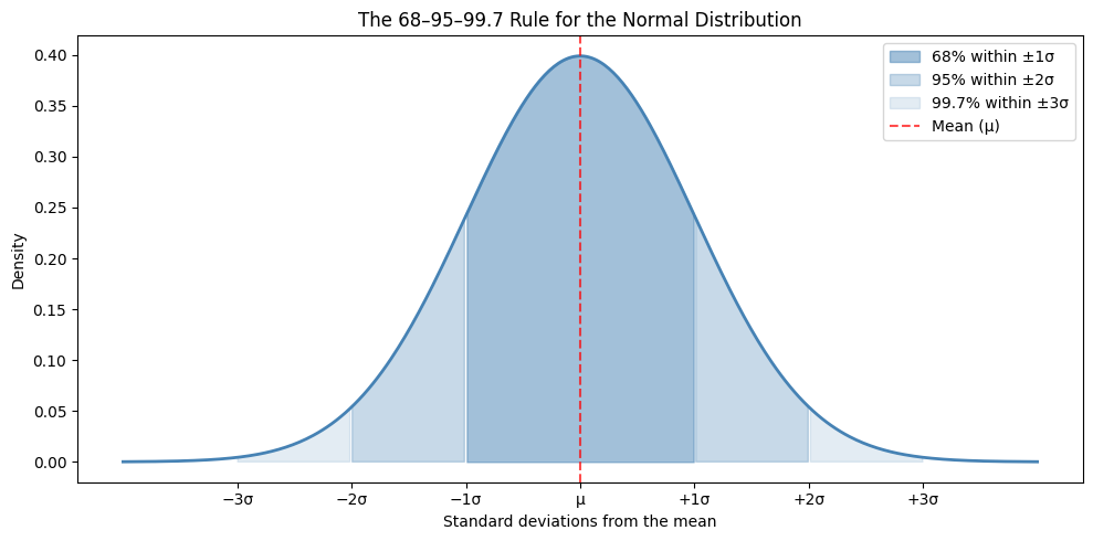
Look at the three bands:
About 68% of the area sits within ±1σ of the mean (the dark blue band)
About 95% sits within ±2σ
About 99.7% sits within ±3σ
These percentages are true for any normal distribution — they don’t depend on what μ or σ are. This pattern is so common it has a name: the 68-95-99.7 rule (or the empirical rule). Worth memorising — we’ll use it constantly.
Tip
Quick sanity check: if you ever see a “normal” histogram where almost nothing falls within ±1σ of the mean, something’s wrong — your distribution probably isn’t normal.
Setting Up#
Most of what we need lives in scipy.stats. Let’s import everything we’ll use:
import numpy as np
import pandas as pd
from scipy import stats
import matplotlib.pyplot as plt
import seaborn as sns
Z-Scores: putting different distributions on the same scale#
Here’s a puzzle. Two students take exams in different subjects:
Alice scored 85 on a maths exam where the class mean was 70 and SD was 10.
Ben scored 90 on an English exam where the class mean was 80 and SD was 5.
Ben scored higher in absolute terms (90 vs 85). But who did relatively better compared to their own classmates? Maths and English exams aren’t directly comparable — different teachers, different classes, different difficulty — so we need a way to put both scores on the same scale.
That’s the job of the z-score. It tells you how many standard deviations a value is from its mean:
Let’s compute Alice’s z-score directly:
# Alice: score 85, class mean 70, SD 10
(85 - 70) / 10
1.5
That’s already the answer: 1.5. Alice scored 1.5 standard deviations above her class mean. Now Ben:
# Ben: score 90, class mean 80, SD 5
(90 - 80) / 5
2.0
Ben’s z-score is 2.0 — two standard deviations above his class mean. So even though Alice’s raw score was lower, Ben did relatively better in his class. The z-score lets us compare apples to oranges.
For the rest of the chapter we’ll do the same calculation in a slightly cleaner way, with named variables — this scales nicely once you start doing many calculations on the same dataset:
x     = 85    # the raw score
mu    = 70    # mean
sigma = 10    # standard deviation

z = (x - mu) / sigma
print("z-score:", z)
z-score: 1.5
Notice that a z-score has no units. It’s a pure ratio — “this many standard deviations from the mean” — which is exactly why it works for comparing across different scales.
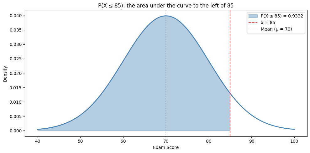
A z-score of 1.5 tells us Alice did well, but how well exactly? What proportion of students did she beat? That’s where norm.cdf() comes in.
Finding Probabilities with norm.cdf()#
The CDF (Cumulative Distribution Function) answers one question: what proportion of values fall at or below a given point? In Python that’s stats.norm.cdf(). The simplest call is:
# Probability of scoring 85 or below in Alice's class (mean 70, SD 10)
stats.norm.cdf(85, loc=70, scale=10)
np.float64(0.9331927987311419)
So 0.9332. Let’s save it to a variable and present it more clearly:
prob_below = stats.norm.cdf(85, loc=70, scale=10)
print("P(score ≤ 85):", round(prob_below, 4))
print("That's", round(prob_below * 100, 1), "% of students")
P(score ≤ 85): 0.9332
That's 93.3 % of students
So Alice did better than about 93% of her class. Not bad!
Visually, cdf is the shaded area to the left of the value — that’s literally all it computes:
Show code cell source
mu, sigma = 70, 10
x = np.linspace(40, 100, 400)
y = stats.norm.pdf(x, mu, sigma)

fig, ax = plt.subplots(figsize=(10, 5))
ax.plot(x, y, color='steelblue', linewidth=2)
ax.fill_between(x, y, where=(x <= 85),
                alpha=0.4, color='steelblue', label='P(X ≤ 85) = 0.9332')
ax.axvline(x=85, color='red', linestyle='--', alpha=0.7, label='x = 85')
ax.axvline(x=mu, color='gray', linestyle=':', alpha=0.5, label='Mean (μ = 70)')
ax.set_xlabel('Exam Score')
ax.set_ylabel('Density')
ax.set_title('P(X ≤ 85): the area under the curve to the left of 85')
ax.legend()
plt.tight_layout()
plt.show()
Note
In stats.norm.cdf(), loc is the mean (μ) and scale is the standard deviation (σ). If you’re working with the standard normal (μ=0, σ=1), you can just pass the z-score directly: stats.norm.cdf(1.5) gives the same answer.
What about the proportion ABOVE a value?#
Here’s where beginners often get tripped up. norm.cdf() always gives you the area to the left. What if you want the area to the right?
The trick: the total area under the curve is 1, so the area above is just 1 - cdf. Watch:
# Probability above 85 = 1 minus probability below 85
1 - stats.norm.cdf(85, loc=70, scale=10)
np.float64(0.06680720126885809)
About 0.0668. Or with a friendly print:
prob_above = 1 - stats.norm.cdf(85, loc=70, scale=10)
print("P(score > 85):", round(prob_above, 4))
print("That's only", round(prob_above * 100, 1), "% of students")
P(score > 85): 0.0668
That's only 6.7 % of students
So a score of 85 is in roughly the top 7% of the class — same conclusion as before, just looked at from the other side.
Warning
A common mistake is using norm.cdf() directly when you want the area above a value. Remember: norm.cdf() always gives you the area below. For “above”, subtract from 1.
Probability between two values#
What proportion scored between 60 and 80? Same trick — take the area below 80, then subtract the area below 60:
# Area between 60 and 80 = (area below 80) − (area below 60)
prob_between = stats.norm.cdf(80, loc=70, scale=10) - stats.norm.cdf(60, loc=70, scale=10)

print("P(60 ≤ score ≤ 80):", round(prob_between, 4))
print("That's", round(prob_between * 100, 1), "% of students")
P(60 ≤ score ≤ 80): 0.6827
That's 68.3 % of students
Wait — 68.3%? That’s the 68-95-99.7 rule in action! The range 60 to 80 is exactly ±1 standard deviation around the mean (70 ± 10), and we’ve just confirmed empirically that about 68% of the area falls within ±1σ.
Notice we can use the same cdf() function to answer three different shapes of question — below, above, between — by combining or subtracting calls. There’s no separate function for each; just one tool used three ways.
Finding Values with norm.ppf() — the inverse question#
norm.cdf() answers: given a value, what’s the probability of being below it?
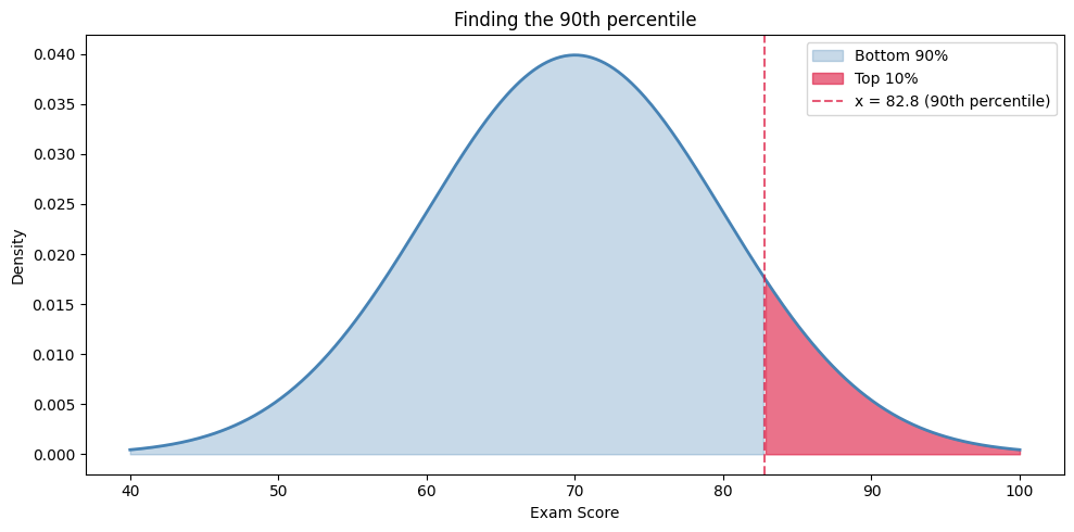
Sometimes you want to flip the question around: given a probability, what’s the value? For example: what score would put a student in the top 10%?
That’s what norm.ppf() does — it’s the inverse of cdf(). The simplest call:
# What score sits at the 90th percentile (top 10%) in Alice's class?
stats.norm.ppf(0.90, loc=70, scale=10)
np.float64(82.815515655446)
Roughly 82.8. Cleaner output:
score_90th = stats.norm.ppf(0.90, loc=70, scale=10)
print("90th percentile cutoff:", round(score_90th, 1))
90th percentile cutoff: 82.8
So a student would need to score about 83 to be in the top 10% of Alice’s class. Visually, that’s the cutoff where the right tail holds 10% of the area:
Show code cell source
mu, sigma = 70, 10
x_critical = stats.norm.ppf(0.90, loc=mu, scale=sigma)
x = np.linspace(40, 100, 400)
y = stats.norm.pdf(x, mu, sigma)

fig, ax = plt.subplots(figsize=(10, 5))
ax.plot(x, y, color='steelblue', linewidth=2)
ax.fill_between(x, y, where=(x <= x_critical),
                alpha=0.3, color='steelblue', label='Bottom 90%')
ax.fill_between(x, y, where=(x >= x_critical),
                alpha=0.6, color='crimson', label='Top 10%')
ax.axvline(x=x_critical, color='crimson', linestyle='--', alpha=0.7,
           label=f'x = {x_critical:.1f} (90th percentile)')
ax.set_xlabel('Exam Score')
ax.set_ylabel('Density')
ax.set_title('Finding the 90th percentile')
ax.legend()
plt.tight_layout()
plt.show()
One special z-score you’ll see everywhere#
Here’s a particular ppf() call that will come up again and again in the rest of this chapter — the z-score that leaves 2.5% of the distribution in each tail:
# z-score with 97.5% of the area below it (i.e. 2.5% in the upper tail)
stats.norm.ppf(0.975)
np.float64(1.959963984540054)
That value — 1.96 — is the basis of every 95% confidence interval you’ll ever build. It’s arguably the most famous number in statistics. Memorise it; you’ll need it constantly.
Why 0.975 and not 0.95? Because we want a two-sided interval. The 5% we’re leaving outside is split into two tails (2.5% in each), so we need the value that leaves 97.5% below it.
z_95 = stats.norm.ppf(0.975)
print("z* for 95% confidence:", round(z_95, 4))
z* for 95% confidence: 1.96
Summary of Normal Distribution Functions#
Function |
What it does |
Example |
|---|---|---|
|
P(X ≤ x) — probability below x |
“What % scored below 85?” |
|
Value at the p-th percentile |
“What score is the 90th percentile?” |
|
Height of the curve at x |
For plotting the distribution |
|
P(Z ≤ z) for the standard normal |
When working with z-scores |
|
z-score at the p-th percentile |
Finding critical values (z*) |
Tip
When using the standard normal distribution (μ=0, σ=1), you can omit loc and scale: stats.norm.cdf(1.96) gives you the same result as stats.norm.cdf(1.96, loc=0, scale=1).
Sampling Distributions and the Central Limit Theorem#
Up until now we’ve focused on the distribution of individual values — one student’s exam score, one baby’s birth weight. But for statistical inference we care about something subtly different: how would our sample mean vary if we’d drawn a different sample?
The thought experiment#
Imagine you randomly sampled 50 babies and computed the average birth weight. You got, say, 7.05 lbs.
Now imagine you took another random sample of 50 babies. The average wouldn’t be exactly 7.05 — it might be 7.12, or 6.98. A third sample might give 7.20.
If you collected hundreds of these sample means and plotted them as a histogram, you’d get a brand-new distribution: the sampling distribution of the mean. This idea — that the sample mean itself has a distribution — is one of the most useful in all of statistics.
Let’s actually simulate it#
We don’t have to imagine. We can do it. To make the result striking, let’s start with a population that is definitely not normal — a flat (uniform) distribution of scores between 0 and 100:
Show code cell source
np.random.seed(42)
population = np.random.uniform(0, 100, 100000)

fig, ax = plt.subplots(figsize=(10, 4))
ax.hist(population, bins=50, color='steelblue', alpha=0.6, edgecolor='white')
ax.set_xlabel('Score')
ax.set_ylabel('Count')
ax.set_title('Population: scores 0–100, distributed UNIFORMLY (not normal)')
plt.tight_layout()
plt.show()
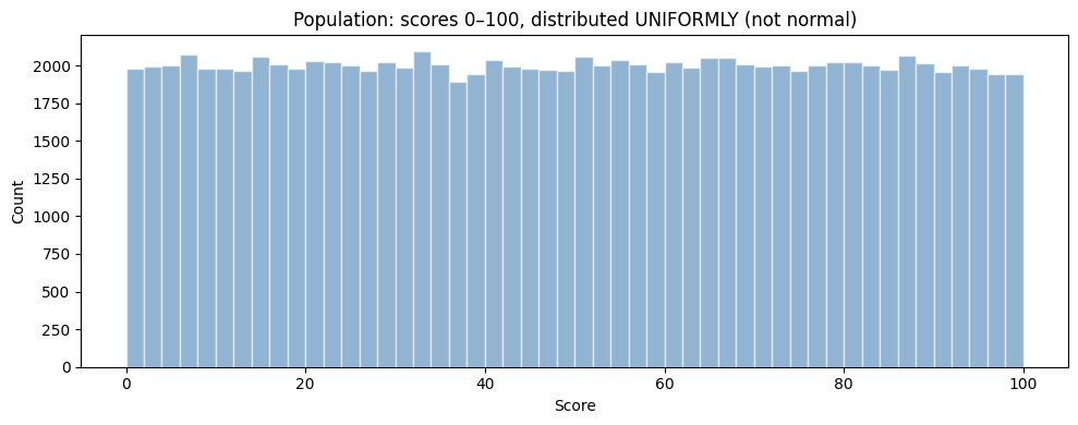
This is our population. Flat as a pancake — far from a bell. The true population mean is 50.
Now let’s take one random sample of 30 scores and compute its mean:
np.random.seed(42)
sample = np.random.uniform(0, 100, 30)
sample.mean()
np.float64(43.859727209743674)
So our first sample mean is around 50, but not exactly. If we drew a different sample, we’d get a slightly different number. Let’s repeat this 1,000 times and store the mean of every single sample:
np.random.seed(42)
sample_means = []

for i in range(1000):
    sample = np.random.uniform(0, 100, 30)
    sample_means.append(sample.mean())

print("Number of sample means collected:", len(sample_means))
print("First five:", np.round(sample_means[:5], 2))
Number of sample means collected: 1000
First five: [43.86 49.64 48.22 49.13 45.6 ]
Each entry of sample_means is the average of a different random sample of 30. Now plot the histogram of these 1,000 sample means:
Show code cell source
fig, ax = plt.subplots(figsize=(10, 4))
ax.hist(sample_means, bins=30, color='steelblue', alpha=0.7, edgecolor='white')
ax.axvline(50, color='red', linestyle='--', label='True population mean (50)')
ax.set_xlabel('Sample mean')
ax.set_ylabel('Frequency')
ax.set_title('Sampling distribution of the mean (1,000 samples, each n=30)')
ax.legend()
plt.tight_layout()
plt.show()
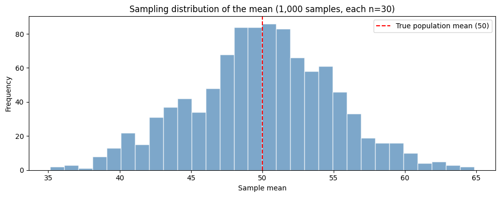
Two things should jump out:
It looks like a bell curve — even though the population we drew from was a flat rectangle.
It’s centred at 50 — the true population mean.
That’s the Central Limit Theorem in action.
The Central Limit Theorem (CLT)#
The CLT tells us three precise things about the sampling distribution of the mean:
It is approximately normal — even when the original data isn’t.
Its centre equals the population mean (μ).
Its spread is σ / √n, where σ is the population standard deviation and n is the sample size.
That third property is so useful it gets its own name — the standard error:
In plain English: the SE is the standard deviation of the sample mean, not of individual values. It tells us how far a typical sample mean is likely to land from the true population mean.
Larger samples give tighter sampling distributions#
Notice that n sits under a square root in the SE formula. That has a non-obvious consequence: to halve the standard error you have to quadruple the sample size. Doubling n only shrinks the SE by about 30%.
We can see this directly. Compare the sampling distribution for n = 10, n = 50, and n = 200:
Show code cell source
fig, axes = plt.subplots(1, 3, figsize=(15, 4), sharex=True, sharey=True)

for ax, n in zip(axes, [10, 50, 200]):
    np.random.seed(42)
    means = [np.random.uniform(0, 100, n).mean() for _ in range(1000)]
    ax.hist(means, bins=30, color='steelblue', alpha=0.7, edgecolor='white')
    ax.axvline(50, color='red', linestyle='--')
    ax.set_title("n = " + str(n) + "\nempirical SE ≈ " + str(round(np.std(means, ddof=1), 2)))
    ax.set_xlabel('Sample mean')

axes[0].set_ylabel('Frequency')
plt.tight_layout()
plt.show()
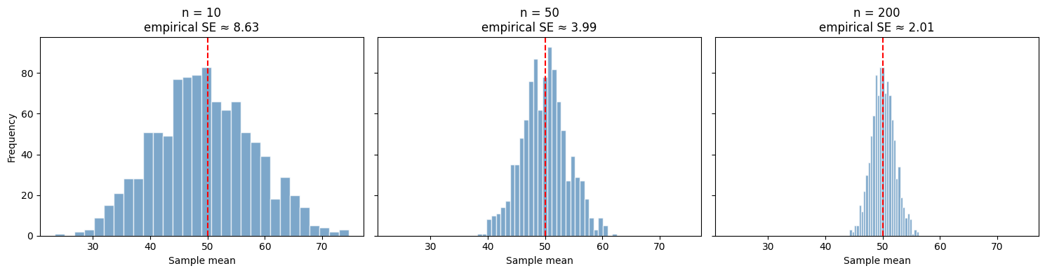
Three things to notice:
All three distributions are bell-shaped — the CLT works regardless of n (as long as n isn’t tiny — say, > 30).
All three are centred at 50 — the true population mean.
The spread shrinks as n grows: from SE ≈ 8.6 (n=10) → ≈ 4.0 (n=50) → ≈ 2.0 (n=200). Quadrupling n roughly halves the SE — exactly what the √n in the formula predicts.
Why this matters#
Here’s the payoff: the CLT lets us use the normal distribution to do inference on means, even when the underlying data is wildly non-normal. That’s why everything we just learned about z-scores, cdf, and ppf keeps coming back — it’s the engine that lets us build the confidence intervals and run the hypothesis tests in the rest of this chapter.
Confidence Intervals#
In the last section we saw that the sample mean has its own distribution — a different sample would have produced a different mean. So when we report “the average birth weight in our sample is 7.05 lbs”, we’re really just giving one possible answer.
Wouldn’t it be more honest to report a range — something like “we’re 95% confident the true average is between 6.26 and 7.06 lbs”? That’s exactly what a confidence interval (CI) gives us.
Every CI follows the same simple template:
What goes into “estimate”, “critical value”, and “standard error” depends on whether we’re dealing with proportions, means, or differences — but the shape is always the same. Let’s build CIs for two cases.
Confidence Interval for a Proportion#
For categorical data — yes/no, premature/not, smoker/nonsmoker — the formula is:
For 95% confidence the critical value is z = 1.96* — the very number we computed in the last section as stats.norm.ppf(0.975).
Example: Proportion of Premature Births#
We have a sample of 50 babies in birth_weights_sample.csv. Each row records the baby’s birth weight (in pounds) and a premature flag (1 = premature, 0 = full term). Let’s build a 95% CI for the true population proportion of premature births, one step at a time.
Step 1 — Load the data and compute the sample proportion:
births = pd.read_csv("https://raw.githubusercontent.com/sakibanwar/python-notes/main/data/birth_weights_sample.csv")

n = len(births)
x = births["premature"].sum()
p_hat = x / n

print("Sample size n =", n)
print("Number premature x =", x)
print("Sample proportion p_hat =", round(p_hat, 4))
Sample size n = 50
Number premature x = 8
Sample proportion p_hat = 0.16
So 8 out of 50 babies in our sample are premature — a sample proportion of 0.16 (or 16%).
Step 2 — Compute the standard error:
se = np.sqrt(p_hat * (1 - p_hat) / n)
print("Standard error:", round(se, 4))
Standard error: 0.0518
The SE is a measure of how much our sample proportion would jiggle around if we kept drawing fresh samples of 50.
Step 3 — Find the critical value:
z_star = stats.norm.ppf(0.975)
print("z* for 95% confidence:", round(z_star, 4))
z* for 95% confidence: 1.96
That’s the famous 1.96 — the z-score that puts 2.5% of the area in each tail.
Step 4 — Combine into the confidence interval:
lower = p_hat - z_star * se
upper = p_hat + z_star * se

print("95% CI: from", round(lower, 4), "to", round(upper, 4))
print("In percentages:", round(lower * 100, 1), "% to", round(upper * 100, 1), "%")
95% CI: from 0.0584 to 0.2616
In percentages: 5.8 % to 26.2 %
So we’re 95% confident the true population proportion of premature births is between about 6% and 26%.
Visually, that’s a range around our point estimate:
Show code cell source
fig, ax = plt.subplots(figsize=(10, 2.5))
ax.errorbar(p_hat, 0,
            xerr=[[p_hat - lower], [upper - p_hat]],
            fmt='o', color='steelblue', capsize=10, markersize=12,
            elinewidth=2, label='95% confidence interval')
ax.axvline(p_hat, color='red', linestyle=':', alpha=0.6, label='Sample p_hat = ' + str(round(p_hat, 2)))
ax.set_xlim(-0.05, 0.5)
ax.set_yticks([])
ax.set_xlabel('Population proportion of premature births')
ax.set_title('95% Confidence Interval')
ax.legend(loc='upper right')
plt.tight_layout()
plt.show()
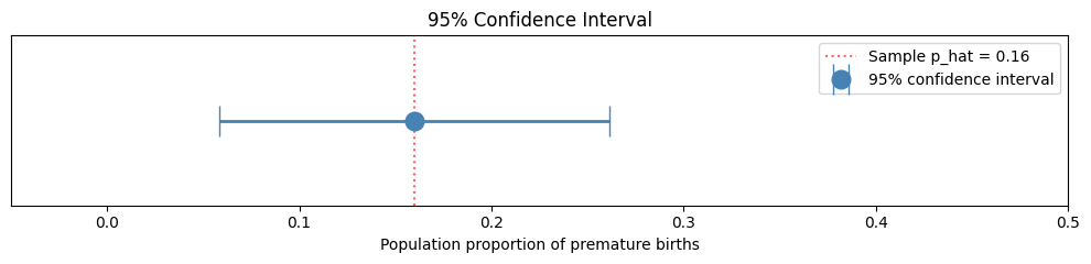
Notice how wide that interval is — from roughly 6% to 26%. With only 50 observations the standard error is large, so we can’t pin the true rate down very precisely. Larger samples produce tighter intervals (remember the √n in the SE denominator). We’ll see this in action with the larger births_smoking.csv dataset later in the chapter.
Note
What does “95% confident” actually mean? It does not mean there’s a 95% probability the true value is in this particular interval. Instead, it means: if we repeated this study many times and constructed a CI each time, about 95% of those intervals would contain the true population proportion. It’s a statement about the method, not about any single interval.
Confidence Interval for a Mean#
For means, the structure is the same but two things change: we use the t-distribution instead of the normal, and we use the sample standard deviation s in place of σ:
Why t instead of z? Because when we estimate σ from the sample (rather than knowing the true value), we introduce a little extra uncertainty. The t-distribution accounts for this with slightly wider tails — especially noticeable for small samples. The critical value t* depends on the degrees of freedom, which is just n - 1.
Example: Average Birth Weight#
Same dataset, different question: build a 95% CI for the true mean birth weight.
Step 1 — Load the data and compute sample statistics:
births = pd.read_csv("https://raw.githubusercontent.com/sakibanwar/python-notes/main/data/birth_weights_sample.csv")
weights = births["weight_lbs"].values

n = len(weights)
x_bar = weights.mean()
s = weights.std(ddof=1)   # ddof=1 = SAMPLE standard deviation

print("n =", n)
print("Sample mean x_bar =", round(x_bar, 3), "lbs")
print("Sample SD s =", round(s, 3))
n = 50
Sample mean x_bar = 6.662 lbs
Sample SD s = 1.401
Tip
The ddof argument relates to degrees of freedom (the “df” you’ve seen in your stats class) — it tells numpy how much to subtract from n when dividing. We used ddof=1 when calculating the standard deviation. That gives us the sample standard deviation (dividing by n − 1). Without ddof=1, numpy divides by n, which gives the population standard deviation. For inference, you almost always want ddof=1.
Step 2 — Standard error:
se = s / np.sqrt(n)
print("Standard error:", round(se, 3))
Standard error: 0.198
Step 3 — Critical value (t this time, not z):**
t_star = stats.t.ppf(0.975, df=n-1)
print("t* for 95% confidence with df =", n-1, ":", round(t_star, 4))
t* for 95% confidence with df = 49 : 2.0096
Step 4 — Combine:
lower = x_bar - t_star * se
upper = x_bar + t_star * se
print("95% CI for mean birth weight:", round(lower, 3), "to", round(upper, 3), "lbs")
95% CI for mean birth weight: 6.264 to 7.06 lbs
So we’re 95% confident the true mean birth weight in the wider population is between about 6.26 and 7.06 lbs.
Note
Notice how t* (≈ 2.01) is just slightly larger than z* (≈ 1.96). That’s the t-distribution’s wider tails kicking in — they make CIs slightly wider to account for the extra uncertainty from estimating σ from the sample. As n grows, t* shrinks toward z*: at n = 100 you’d see t* ≈ 1.984; by n = 1,000 it’s basically 1.96.
What’s next#
You now have the two pillars of estimation: the Central Limit Theorem (which tells us how sample statistics vary) and confidence intervals (which give us a sensible range for the population value). With these in hand, we can move on to the second big task of statistical inference: decision-making.
In the next chapter — Statistical Inference: Hypothesis Testing — we’ll see how to use the same machinery to ask yes/no questions about populations: is there really a difference between two groups? is a sample proportion meaningfully different from some baseline? Each question becomes a hypothesis test with a p-value telling us how strongly the data support a conclusion.
Summary#
Here’s a quick reference for the foundational tools we built in this chapter.
Normal Distribution Functions#
Function |
Purpose |
Example |
|---|---|---|
|
P(X ≤ x) |
“What % scored below 85?” |
|
Value at percentile p |
“What score is the 90th percentile?” |
|
Standard normal P(Z ≤ z) |
“What’s the area to the left of z = 1.96?” |
|
z* for 95% CI |
Returns 1.96 |
Confidence Interval Formulas#
Parameter |
Formula |
Critical value |
|---|---|---|
Proportion |
p̂ ± z* × √(p̂(1−p̂)/n) |
z* = |
Mean |
x̄ ± t* × s/√n |
t* = |
Key Takeaways#
The normal distribution underpins most inference — learn
norm.cdf()andnorm.ppf()inside out.Remember:
norm.cdf()gives the area below. For “above”, use1 − norm.cdf().The Central Limit Theorem says the sampling distribution of the mean is approximately normal even if the underlying data isn’t — this is what lets us use the normal distribution for inference on means.
Confidence intervals give a range of plausible values — not a “95% probability” of containing the truth. They’re a statement about the method, not any single interval.
The standard error has √n in the denominator, so quadrupling the sample size halves the SE.
Exercises#
Exercise 32
Exercise 1: The Normal Distribution
The heights of adult males in the UK are approximately normally distributed with mean μ = 175 cm and standard deviation σ = 7 cm.
What proportion of men are taller than 185 cm?
What proportion of men are between 168 cm and 182 cm?
How tall does a man need to be to be in the tallest 5%?
What height marks the 25th percentile?
Solution to Exercise 32
from scipy import stats

mu = 175
sigma = 7

# 1. Proportion taller than 185 cm
prop_above_185 = 1 - stats.norm.cdf(185, loc=mu, scale=sigma)
print("1. Proportion taller than 185 cm: ", round(prop_above_185, 4), "= about", round(prop_above_185 * 100, 1), "%")

# 2. Proportion between 168 and 182 cm
prop_between = stats.norm.cdf(182, loc=mu, scale=sigma) - stats.norm.cdf(168, loc=mu, scale=sigma)
print("2. Proportion between 168 and 182 cm: ", round(prop_between, 4), "= about", round(prop_between * 100, 1), "%")

# 3. Height for tallest 5% (95th percentile)
height_95 = stats.norm.ppf(0.95, loc=mu, scale=sigma)
print("3. Tallest 5% threshold: ", round(height_95, 1), " cm")

# 4. 25th percentile
height_25 = stats.norm.ppf(0.25, loc=mu, scale=sigma)
print("4. 25th percentile height: ", round(height_25, 1), " cm")
1. Proportion taller than 185 cm: 0.0766 (7.7%)
2. Proportion between 168 and 182 cm: 0.6827 (68.3%)
3. Tallest 5% threshold: 186.5 cm
4. 25th percentile height: 170.3 cm
Exercise 33
Exercise 2: Confidence Interval for a Proportion
In a survey of 500 university students, 320 said they use public transport to get to campus.
Calculate the sample proportion
Calculate the standard error
Construct a 95% confidence interval for the true proportion
Would a 99% confidence interval be wider or narrower? Calculate it to verify.
Solution to Exercise 33
import numpy as np
from scipy import stats

n = 500
x = 320
p_hat = x / n

# 1. Sample proportion
print("1. Sample proportion: ", round(p_hat, 4), "= about", round(p_hat * 100, 1), "%")

# 2. Standard error
se = np.sqrt(p_hat * (1 - p_hat) / n)
print("2. Standard error: ", round(se, 4))

# 3. 95% confidence interval
z_95 = stats.norm.ppf(0.975)
lower_95 = p_hat - z_95 * se
upper_95 = p_hat + z_95 * se
print("3. 95% CI: (", round(lower_95, 4), ", ", round(upper_95, 4), ")")

# 4. 99% confidence interval
z_99 = stats.norm.ppf(0.995)
lower_99 = p_hat - z_99 * se
upper_99 = p_hat + z_99 * se
print("4. 99% CI: (", round(lower_99, 4), ", ", round(upper_99, 4), ")")
print("   The 99% CI is WIDER — more confidence requires a wider range")
1. Sample proportion: 0.6400 (64.0%)
2. Standard error: 0.0215
3. 95% CI: (0.5979, 0.6821)
4. 99% CI: (0.5847, 0.6953)
   The 99% CI is WIDER — more confidence requires a wider range
Appendix: How the Datasets Were Created#
The datasets used in this chapter were generated using Python’s numpy.random module to simulate realistic data. This appendix explains how each was created, so you can understand the data and learn how to simulate your own.
Birth Weights Sample (birth_weights_sample.csv)#
A sample of 50 babies. Each row records the baby’s birth weight (drawn from a normal distribution with mean 7.0 lbs and standard deviation 1.5 lbs) and a premature flag (1 = premature, 0 = full term). We deliberately link “premature” to the lower birth weights — in real data, premature babies tend to be smaller than full-term ones.
import numpy as np
import pandas as pd

np.random.seed(42)  # Makes the random weights reproducible

# Generate weights
weights = pd.DataFrame({
    'weight_lbs': np.random.normal(7.0, 1.5, 50).round(2)
})

# Mark the 8 lowest-weight babies as premature (16% premature rate)
weights = weights.sort_values('weight_lbs').reset_index(drop=True)
weights['premature'] = 0
weights.loc[:7, 'premature'] = 1     # first 8 rows after sorting

# Shuffle so the rows aren't ordered by weight
weights = weights.sample(frac=1, random_state=123).reset_index(drop=True)

weights.to_csv('birth_weights_sample.csv', index=False)
What’s happening:
np.random.seed(42)ensures you get the same “random” weights every time — this is called reproducibilitynp.random.normal(7.0, 1.5, 50)draws 50 values from a normal distribution with mean 7.0 and standard deviation 1.5After sorting by weight, the 8 lightest babies are flagged premature — this gives the dataset a realistic correlation between low birth weight and prematurity
The final shuffle (with a different
random_state) mixes the rows back up so the data isn’t sorted by weight